Stock markets are hard to predict because they depend on a tremendous amount of factors including historical data and economic news. Let’s try to improve the explanation of stock markets by including some related search terms from the Google search engine. This work aims at evaluating the use of those search data in nowcasting the stock market. We want to answer the following research question:
- What are the best models to predict the near term price movement of stock markets, more specifically the S&P 500 index?
- Can we improve our predictions using Google Trends? If yes, to what extent?
- Which Google Trends keywords are most relevant in explaining stock market price variations and why?
This work is based on the paper Predicting the Present with Google Trends 1 from HYUNYOUNG CHOI and HAL VARIAN. The original paper explains how Google Trends help improve forecasts with a baseline model. In contrast, we will explore different prediction models to choose the optimal one to forecast the price movement of one of the most popular US Stock index, the S&P 500. Then, Google Trends data will be introduced to see if we can improve these predictions. A Google Trends keywords selection will be performed beforehand to keep the most relevant ones. In the end, we’ll have the possibility to test our models in predicting the stock prices of recession periods from the S&P 500.
Predicting the Present with Google Trends
Let’s get started with a bit of context. We will now give a short and general summary of the work done in the original paper. The authors propose to use google trends data to improve the predicitions of several economic indicators. The table below shows the 4 economic series considered and the Google Trends term associated:
| Economic indicator | Google Trends |
|---|---|
| Automobile sales | Trucks & SUVs, Automotive Insurance |
| Unemployment claims | Jobs, Welfare & Unemployment |
| Hong Kong arrivals | Hong Kong (by countries of origin) |
| Consumer confidence | Crime & Justice, Trucks & SUVs, Hybrid & Alternative Vehicles |
The Google Trends data are time series measuring of the number of Google research for the subject considered.
For each of those time series, the authors compare the usage of expanding window Auto-Regressive models with and without including the related search terms. The models have either a lag of -1 or a lag of -1 and -12. The series of economic indicators can be pre-processed to be log-transformed and are sometimes seasonally adjusted.
Their results show that including the Google Trends data reduces the errors in predictions by 5 to 20 percent.
Extension to stock markets
We now present our work related to stock market data. Let’s start with a description of the data used.
Data
There are two main datasets. The first one is the economic indicator of interest, the S&P 500 price. And the second one is Google Trends data. These two data sets are time series ranging from early 2004 to nowadays. The data sets are available on daily data points but we will resample them to keep only the last weekly point so that the data has weekly points.
S&P 500
The S&P 500 is a stock market index that measures the stock performance of 500 large companies listed on stock exchanges in the United States. This index is one of the most used to represent US financial markets.
We use the S&P500 data for our analysis, it was downloaded from Yahoo Finance. The data is a table containing the daily values of the S&P500, we have 6 value for each working date (all in $):
- Open: the value of the stock at the opening
- High: the highest value of the stock during the day
- Low: the lowest value of the stock during the day
- Close: the value of the stock at closing
- Adjusted Close: the value of the stock at closing (corrections for stock splits, dividends, and rights offerings)
- Volume: The total amount traded
Let’s start the data exploration for the S&P 500. We will consider the Adjusted Close value for the stock as it is the standard benchmark used by investors to track its performance over time 2.
We first plot the evolution of the Adjusted Close over the year. We will refer to this as the signal.
We can see the big drop in 2008/2009 from the subprime crisis and also around March/April 2020 with the first COVID-19 wave.
Seasonality
We then use a simple decomposition tool from statsmodel to decompose our signal. We choose to use the additive model and our signal is then decomposed as:

with
- Y[t] is the original signal, Adjusted Close for us
- T[t] is the trend signal
- S[t] is the seasonal signal
- e[t] is the residual signal
The results can be seen in the figure below:
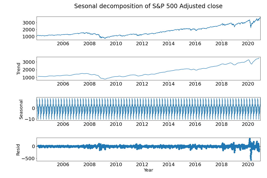
There seems to be a monthly seasonality. We can see this from all the recurring up and down in a year. Which seems to correlate with a monthly period.
Autocorrelation
Let’s now look at the partial autocorrelation function of our signal. It will be important to confirm the usage of Auto-Regressive models. The h order (lag) partial autocorrelation is defined by

Now we show the partial autocorrelation function up to the 20th order.
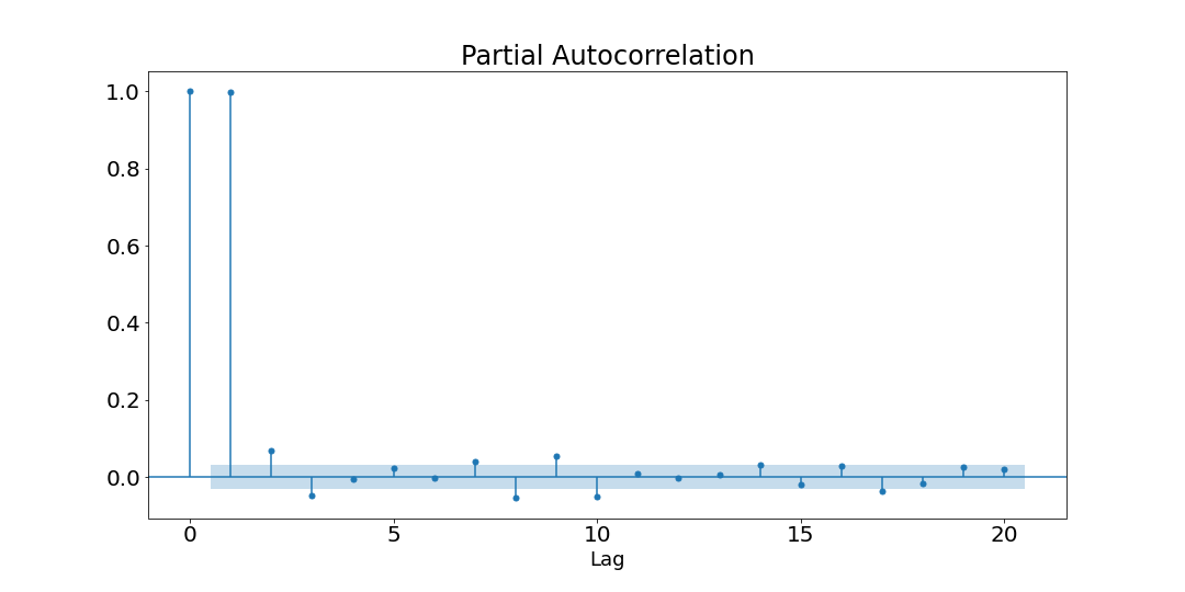
Since the function becomes silent after the first order, then a simple Autoregressive model with a lag of 1 would be sufficient to make predictions 3. However, we will look at more complex models.
First difference
Finally, let’s have a look at the first difference of the signal. This is for each time t we compute the difference of the signal at time t and t-1:
 . We show the resulting signal below:
We can see exponential behavior in 2008/2009 and mainly in March/April 2020. We had similar behavior in the residuals in the seasonality decomposition. To counter this we will use the logarithm of the Adjusted Close to have a more smooth behavior. Note that in the original paper, the authors used the logarithm of the target variable so this is consistent with their results. The new signal, which will use in our model, is shown below:
Google Trends
Let’s now continue our data exploration with the Google Trends data. The main challenge will be to find the relevant Google Trends to include in our models.
Generalities
First, let’s explain what are the Google Trends data, we have briefly mentioned them in the explanation of the original paper but what are they really? Google Trends is a tool developed by Google with analyzes Google searches and determine how many searches were done over a certain period of time. It is up to the user to define the subject for searches and the time window.
When searching for a term on the Google Trends website, the user will have a graph showing the term’s popularity on the selected time frame. The numbers reflect how many searches have been done for the particular term relative to all Google searches. Thus the numbers are not absolute search volume. Also, the numbers on the graph are normalized so that the highest point has a value of 100. A downwards trend means that the search term’s relative popularity to other terms is decreasing, not necessarily that the total (absolute) number of search, for that term, are decreasing.
Below is displayed an example of the data for the search term “stocks”
The data is available to use on Google Trends
Google Trends data are available daily, we will collect them weekly to match the S&P 500 data which we will sample by week. It is also important to note that trend data can be limited to some specific geographical position. In our work we will only use trends data from the United States as the target we want to predict, the S&P 500 is based in the US.
Our keywords
Now that we learned what is the Google Trends data, comes one of our research questions: What are the search terms to include to improve the nowcasting of financial markets?
We selected search terms based on Quantifying Trading Behavior in Financial Markets Using Google Trends 4 and obtained a looooong list of search terms. We only show a few of them here, for completeness have a look at the code :).
Search terms used include: “debt”, “employment”, “economics”, “cancer”, “crisis”, “hedge”, “greed”, “finance”, “risk”, “success”, “movie”, “environment”, “buy spdr”.
We also included search terms for companies in the S&P 500 such as “apple”, “google”, “walmart”, “mastercard”, “walt disney”, “coca cola”, “intel”, “cisco”, “oracle”.
We now have our list of terms to include in our predictions, of course, we won’t use all of them. An important part of the work will now to find the most relevant ones. First, we will look at the best model to use on the S&P500 and then include our google trends to see if there is an improvement.
Model selection
To have a baseline prediction of S&P 500, against which we will compare. We use a simple Auto-Regressive (AR) model with two lags, one of 4 and (because 4 weeks correspond to one month lag) and one of 52 (because 52 weeks corresponds to one year lag). The model is then x[t] = x[t-4] + x[t-52], where x is the log Adjusted Close.
As in the original paper, we decided to implement the rolling windows models. The goal of the models is to predict with out-sample, say we want to predict for time t, if the model has a window size of k, it works as follow:
- fit the AR model using data from time t-k-1 to t-1.
- predict the value at time t using the fitted AR model.
The model selection problem (question 1 of our research questions) is then to find the best window size, k, to best predict the S&P 500. We iterated on various window sizes from 7 to 30 and picked the model which has the lowest Mean Absolute Error (MAE). We obtained an MAE of 2.825 for a window size of 8.
Adding Trends to model
Overall
The idea for predicting with Google Trends is the same. We fit a model with previous points and we include the trend terms at time t, the AR model is x[t] = x[t-4] + x[t-52] + trends[t].
We now need to select the best trend terms to include in our model. For this, we used the selectKBest function from sklearn. Combining with the f_regression function, then we can find the terms with the lowest p-value. This will give us the terms which are the best correlated with the S&P 500.
To find the best model which predicts the S&P 500, we iterated on both the best window size and the number of trends to include.
We found that that the model with the lowest Mean Absolute Error (MAE) was with a window of 8 and with the 37 best-correlated terms, giving an MAE of 2.2596. Some of the terms are:
“mastercard”, “hedge”, “finance”, “berkshire”, “home depot”, “short sell”, “leverage”, “facebook”, “amazon”, “risk”, “nasdaq”, “paypal”, “procter and gamble”, “intel”, “water”, “fond”, “money”, “rich”, “oracle”, “j p morgan”, “loss”, “house”, “gain”, “gross”, “microsoft”, “crisis” ,”inflation”, “adobe”, “headlines”, “at&t”, “nvidia”, “oil”, “war”, “unemployment”, “opportunity”, “health”, “mcdonalds”, and “return”.
We can see that the best terms mostly make sense. We have some big actors of the S&P 500 (facebook, amazon,…) which are so big that they probably highly influence the S&P 500. There are also some financial terms such as short sell, leverage, return,…
The following plot gives an insight about the link between the K_score and the popularity of a keyword in terms of number of hits on Financial Times and Google. The bigger the bubble is, the better it predicts the S&P500.
We now display our best model without trends and the one with the trends.
We can see that our model with the trends has outperformed the base-model by 20.01%, this is good news and consistent with the results from the original paper and proves that using trends term can improve nowcasting.
As in the original paper, we will also look at some turning points.
Turning points
We next decided to investigate some turning points in the S&P signal. We picked them manually, the turning periods are displayed in the next table with their corresponding start and end dates :
| Start | End |
|---|---|
| 2008-08-15 | 2008-11-01 |
| 2009-02-01 | 2009-03-01 |
| 2010-04-20 | 2010-07-20 |
| 2011-07-15 | 2011-10-15 |
| 2015-08-01 | 2015-10-01 |
| 2016-01-01 | 2016-03-01 |
| 2018-11-20 | 2019-01-01 |
| 2020-02-15 | 2020-04-01 |
We show the corresponding periods in the next figure.
The next table summarizes the results. We use again the moving window regression, like for the overall S&P 500 series.
| Start | End | MAE base | MAE trends | 1-ratio |
|---|---|---|---|---|
| 2008-08-15 | 2008-11-01 | 0.123019 | 0.048421 | 60.63% |
| 2009-02-01 | 2009-03-01 | 0.074313 | 0.055064 | 25.90% |
| 2010-04-20 | 2010-07-20 | 0.047212 | 0.031839 | 32.56% |
| 2011-07-15 | 2011-10-15 | 0.075219 | 0.044836 | 40.39% |
| 2015-08-01 | 2015-10-01 | 0.035376 | 0.027221 | 23.05% |
| 2016-01-01 | 2016-03-01 | 0.029385 | 0.022237 | 24.32% |
| 2018-11-20 | 2019-01-01 | 0.053082 | 0.049273 | 7.174% |
| 2020-02-15 | 2020-04-01 | 0.165429 | 0.071638 | 56.69% |
We can see that we have consistenly improved the Mean Absolute Error. And the results are globally better than the overall results. Recall we improved by 20.01% for the whole data set. Here we are almost always higher and some improvement are very good (>50%). Overall the improvement on the recession periods is 33.84% The results were similar in the original paper but had less extreme improvments.
Conclusion
We have found the best Auto-Regressive rolling window model, with a window of 8. The Mean Absolute Error of this baseline model was 2.824. We were able to decrease Error to 2.259 by including the 37 most correlated Google Trends search terms from our list. Looking at the most relevant terms, we globally can see why they explain some variations of the S&P 500. Most of the terms are big companies from the S&P 500 which probably has a certain influence on the stock value, we also have some financial vocabulary. It seems logical to predict financial movements with financial terms probably searched by the persons interested in stock trading.
Another option could have been to use a more restrained stock market (S&P500 is quite broad) which may give even better results.
A last part of this project could be to make investment recommendations based on the prediction of a fall in stock price (we could set a certain threshold) and see how well our investment recommendation system would work, and how much money we could make from 2004 to 2020. Would we recommend our model to a friend looking forward investing his money?
References
1. H. Choi, H. Varian, Predicting the Present with Google Trends, Economic record, 2012.
2. Will Kento, Closing Price, investopedia.com, last updated Aug 22, 2019.
3. STAT-510 Applied Time Series Analysis, 2.2 Partial Autocorrelation Function (PACF), investopedia.com, last updated Aug 22, 2019.
4. Tobias Preis, Helen Susannah Moat & H. Eugene Stanley, Quantifying Trading Behavior in Financial Markets Using Google Trends, nature.com, published: 25 April 2013